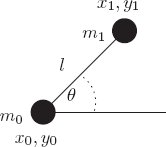
In this exercise we will recapitulate the derivation of the Lagrangian for constrained systems for a particular simple system. Consider two massive particles in the plane constrained by a massless rigid rod to remain a distance l apart, as in figure 1.5. There are apparently four degrees of freedom for two massive particles in the plane, but the rigid rod reduces this number to three. We can uniquely specify the configuration with the redundant coordinates of the particles, say $x_0(t)$, $y_0(t)$ and $x_1(t)$, $y_1(t)$. The constraint $(x_1(t) − x_0(t))^2 + (y_1(t) − y_0(t))^2 = l^2$ eliminates one degree of freedom. Figure 1.5 a. Write Newton’s equations for the balance of forces for the four rectangular coordinates of the two particles, given that the scalar tension in the rod is $F$. b. Write the formal Lagrangian $\mathbf{L}(t;x_0,y_0,x_1,y_1,F;\dot{x}_0,\dot{y}_0,\dot{x}_1,\dot{y}_1,\dot{F})$ such that Lagrange’s equations will yield the Newton’s equations you derived in part a. Restating Eq. 1.93 from the book: This is a Lagrangian that can reproduce Newton’s equations for particles constrained by a fixed-distance constraint using force $F_{\alpha\beta}$. For the dumb-bell, the Lagrangian is These equations of motion are equivalent to the Newtonian equations derivated initially, along with the constraint equation 1.21 c. Make a change of coordinates to a coordinate system with center of mass coordinates $x_{CM}$, $y_{CM}$, angle $\theta$, distance between the particles $c$, and tension force $F$. Write the Lagrangian in these coordinates, and write the Lagrange equations. Mass $m_0$ is at a distance $\frac{m_1 c}{m_0 + m_1}$ from the center of mass and $m_1$ is at a distance $\frac{m_0 c}{m_0 + m_1}$ from the center of mass. Therefore the change of coordinates can be defined as: We can use the From the first two equations, the acceleration of the center of mass is zero. From the 5th equation, we can deduce that $c(t) = l$ and therefore, $Dc = 0$ and $D^2 c = 0$. 1.21d. You may deduce from one of these equations that $c(t) = l$. From this fact we get that $D c = 0$ and $D^2 c = 0$. Substitute these into the Lagrange equations you just computed to get the equation of motion for $x_{CM}$, $y_{CM}$, $\theta$. The third equation now reduces to $\ddot{\theta} = 0$. The fourth equation has the quantity $\frac{m_0 m_1}{m_0 + m_1}$ which is called the “reduced mass” in a Newtonian two-body problem. (). Substituting the reduced mass as $m$ in the fourth EOM, we get: This expression is very similar to the expression for centrifugal force. 1.21e. Make a Lagrangian ($= T − V$) for the system described with the irredundant generalized coordinates $x_{CM}$, $y_{CM}$, $\theta$ and compute the Lagrange equations from this Lagrangian. They should be the same equations as you derived for the same coordinates in part d. We define a Lagrangian for two free particles with masses $m_0$ and $m_1$ and then apply a coordinate transformation to the irredundant coordinates using These equations of motion are identical to the ones obtained in part d.Exercise 1.21: A dumbbell
(defn L-dumbbell [m0 m1 l]
    (fn [[_, [x0, y0, x1, y1, F], [vx0, vy0, vx1, vy1, dF]]]
        (let [T1 (* 1/2 m0 (+ (square vx0) (square vy0)))
              T2 (* 1/2 m1 (+ (square vx1) (square vy1)))
              dx (- x1 x0)
              dy (- y1 y0)
              dist (+ (square dx) (square dy))
              F-by-2l (/ F (* 2 l))]
        (+ T1 T2
           (* F-by-2l (- dist (square l)))
           )
    )
))

(rendermd (let [L (L-dumbbell 'm_0 'm_1 'l)
            state (up (literal-function 'x_0) (literal-function 'y_0) (literal-function 'x_1) (literal-function 'y_1) (literal-function 'F))
            local ((Gamma state) 't)
            ]
           (L local)))
;; Deriving Lagrange equations for L-dumbbell

(def eom-dumbbell (Lagrange-equations (L-dumbbell 'm_0 'm_1 'l)))

(rendertexvec (let [state (up (literal-function 'x_0) (literal-function 'y_0)
                              (literal-function 'x_1) (literal-function 'y_1)
                              (literal-function 'F))]
            ((eom-dumbbell state) 't)))
F->C coordinate change function to derive the new Lagrangian.;; Coordinate transform from CM-coordinates to rectangular
(defn CM->rect [m0 m1]
(fn [[_, [x_cm, y_cm, theta, c, F], _ ]]
(let [total-mass (+ m0 m1)
m0dist (* c (/ m1 total-mass))
m1dist (* c (/ m0 total-mass))
]
(up
(- x_cm (* m0dist (cos theta)))
(- y_cm (* m0dist (sin theta)))
(+ x_cm (* m1dist (cos theta)))
(+ y_cm (* m1dist (sin theta)))
F
)
)
))
(defn L-dumbbell-CM [m0 m1 l]
(fn [q-prime]
((compose (L-dumbbell m0 m1 l) (F->C (CM->rect m0 m1)))
q-prime)))
(rendermd
(let [L (L-dumbbell-CM 'm_0 'm_1 'l)
state (up (literal-function 'x_CM)
(literal-function 'y_CM)
(literal-function 'theta)
(literal-function 'c)
(literal-function 'F))
local ((Gamma state) 't)
]
(L local)
))
;; Computing Lagrange Equations
(def eom-dumbbell-cm (Lagrange-equations (L-dumbbell-CM 'm_0 'm_1 'l)))
(rendertexvec (let [state (up (literal-function 'x_CM) (literal-function 'y_CM)
                              (literal-function 'theta)
                              (literal-function 'c)
                              (literal-function 'F))]
            ((eom-dumbbell-cm state) 't)))
;; Substituting $c(t) = l$ in the EOMs, we get:
(rendertexvec (let [state (up (literal-function 'x_CM) (literal-function 'y_CM)
                              (literal-function 'theta)
                              (fn [t] 'l)
                              (literal-function 'F))]
            ((eom-dumbbell-cm state) 't)))
F->C.;; Lagrangian with just the end particles
(defn L-free-two-particles [m0 m1]
(fn [[_, _, [vx0 vy0 vx1 vy1]]]
(let [T0 (* 1/2 m0 (+ (square vx0) (square vy0)))
T1 (* 1/2 m1 (+ (square vx1) (square vy1)))]
(+ T0 T1)
)))
;; Coordinate transform with irredundant coordinates (unlike in part d, no "c" or "F" here)
(defn dumbbell->rect [m0 m1 l]
(fn [[_, [x_cm, y_cm, theta], _ ]]
(let [total-mass (+ m0 m1)
m0dist (* l (/ m1 total-mass))
m1dist (* l (/ m0 total-mass))
]
(up
(- x_cm (* m0dist (cos theta)))
(- y_cm (* m0dist (sin theta)))
(+ x_cm (* m1dist (cos theta)))
(+ y_cm (* m1dist (sin theta)))
)
)
))
(defn L-dumbbell-part-e [m0 m1 l]
(fn [q-prime]
((compose (L-free-two-particles m0 m1) (F->C (dumbbell->rect m0 m1 l)))
q-prime)))
(rendermd
(let [L (L-dumbbell-part-e 'm_0 'm_1 'l)
state (up (literal-function 'x_CM)
(literal-function 'y_CM)
(literal-function 'theta))
local ((Gamma state) 't)
]
(L local)
))
;; Computing Lagrange Equations
(def eom-dumbbell-part-e (Lagrange-equations (L-dumbbell-part-e 'm_0 'm_1 'l)))
(rendertexvec (let [state (up (literal-function 'x_CM) (literal-function 'y_CM)
                              (literal-function 'theta))]
            ((eom-dumbbell-part-e state) 't)))
$$
\begin{align}
m_0 \ddot{x}_0 &= F \cos\theta = F \frac{x_1 - x_0}{l}\\
m_0 \ddot{y}_0 &= F \sin\theta = F \frac{y_1 - y_0}{l}\\
m_1 \ddot{x}_1 &= -F \cos\theta = -F \frac{x_1 - x_0}{l}\\
m_1 \ddot{y}_1 &= -F \sin\theta = -F \frac{x_1 - x_0}{l} \\
\end{align}
$$
$$
L(t; x, F; \dot{x}, \dot{F}) = \sum_\alpha \frac{1}{2}m_\alpha\mathbf{\dot{x}_\alpha}^2 - V(t,x) + \sum_{\{\alpha,\beta | \alpha<\beta, \beta\leftrightarrow\alpha\}} \frac{F_{\alpha\beta}}{2l_{\alpha\beta}}[ (\mathbf{x_\beta}(t) - \mathbf{x_\alpha}(t))^2 - l_{\alpha\beta}^2 ] \tag{1.93}
$$
$$
L = \frac{1}{2} \left(m_0 (\dot{x_0}^2 + \dot{y_0}^2) + m_1 (\dot{x_1}^2 + \dot{y_1}^2) \right) + \frac{F}{2l}[ (x_1 - x_0)^2 + (y_1 - y_0)^2 - l^2 ]
$$
$$
\frac{\frac{1}{2}\,l\,m_0\,{\left(Dx_0\left(t\right)\right)}^{2} + \frac{1}{2}\,l\,m_0\,{\left(Dy_0\left(t\right)\right)}^{2} + \frac{1}{2}\,l\,m_1\,{\left(Dx_1\left(t\right)\right)}^{2} + \frac{1}{2}\,l\,m_1\,{\left(Dy_1\left(t\right)\right)}^{2} + \frac{-1}{2}\,{l}^{2}\,F\left(t\right) + \frac{1}{2}\,F\left(t\right)\,{\left(x_1\left(t\right)\right)}^{2} - F\left(t\right)\,x_1\left(t\right)\,x_0\left(t\right) + \frac{1}{2}\,F\left(t\right)\,{\left(x_0\left(t\right)\right)}^{2} + \frac{1}{2}\,F\left(t\right)\,{\left(y_1\left(t\right)\right)}^{2} - F\left(t\right)\,y_1\left(t\right)\,y_0\left(t\right) + \frac{1}{2}\,F\left(t\right)\,{\left(y_0\left(t\right)\right)}^{2}}{l}
$$
\begin{pmatrix}\displaystyle{\frac{l\,m_0\,{D}^{2}x_0\left(t\right) + F\left(t\right)\,x_1\left(t\right) - F\left(t\right)\,x_0\left(t\right)}{l}} \cr \cr \displaystyle{\frac{l\,m_0\,{D}^{2}y_0\left(t\right) + F\left(t\right)\,y_1\left(t\right) - F\left(t\right)\,y_0\left(t\right)}{l}} \cr \cr \displaystyle{\frac{l\,m_1\,{D}^{2}x_1\left(t\right) - F\left(t\right)\,x_1\left(t\right) + F\left(t\right)\,x_0\left(t\right)}{l}} \cr \cr \displaystyle{\frac{l\,m_1\,{D}^{2}y_1\left(t\right) - F\left(t\right)\,y_1\left(t\right) + F\left(t\right)\,y_0\left(t\right)}{l}} \cr \cr \displaystyle{\frac{\frac{1}{2}\,{l}^{2} + \frac{-1}{2}\,{\left(x_1\left(t\right)\right)}^{2} + x_1\left(t\right)\,x_0\left(t\right) + \frac{-1}{2}\,{\left(x_0\left(t\right)\right)}^{2} + \frac{-1}{2}\,{\left(y_1\left(t\right)\right)}^{2} + y_1\left(t\right)\,y_0\left(t\right) + \frac{-1}{2}\,{\left(y_0\left(t\right)\right)}^{2}}{l}}\end{pmatrix}
$$
\begin{align}
x_0 = x_{CM} - \frac{m_1 c}{m_0 + m_1} \cos{\theta} \\
y_0 = y_{CM} - \frac{m_1 c}{m_0 + m_1} \sin{\theta} \\
x_1 = x_{CM} + \frac{m_0 c}{m_0 + m_1} \cos{\theta} \\
y_1 = y_{CM} + \frac{m_0 c}{m_0 + m_1} \sin{\theta} \\
\end{align}
$$
$$
\frac{l\,m_0\,m_1\,{\left(c\left(t\right)\right)}^{2}\,{\left(D\theta\left(t\right)\right)}^{2} + l\,{m_0}^{2}\,{\left(Dx_{CM}\left(t\right)\right)}^{2} + l\,{m_0}^{2}\,{\left(Dy_{CM}\left(t\right)\right)}^{2} + l\,m_0\,m_1\,{\left(Dc\left(t\right)\right)}^{2} + 2\,l\,m_0\,m_1\,{\left(Dx_{CM}\left(t\right)\right)}^{2} + 2\,l\,m_0\,m_1\,{\left(Dy_{CM}\left(t\right)\right)}^{2} + l\,{m_1}^{2}\,{\left(Dx_{CM}\left(t\right)\right)}^{2} + l\,{m_1}^{2}\,{\left(Dy_{CM}\left(t\right)\right)}^{2} - {l}^{2}\,m_0\,F\left(t\right) - {l}^{2}\,m_1\,F\left(t\right) + m_0\,F\left(t\right)\,{\left(c\left(t\right)\right)}^{2} + m_1\,F\left(t\right)\,{\left(c\left(t\right)\right)}^{2}}{2\,l\,m_0 + 2\,l\,m_1}
$$
\begin{pmatrix}\displaystyle{m_0\,{D}^{2}x_{CM}\left(t\right) + m_1\,{D}^{2}x_{CM}\left(t\right)} \cr \cr \displaystyle{m_0\,{D}^{2}y_{CM}\left(t\right) + m_1\,{D}^{2}y_{CM}\left(t\right)} \cr \cr \displaystyle{\frac{m_0\,m_1\,{\left(c\left(t\right)\right)}^{2}\,{D}^{2}\theta\left(t\right) + 2\,m_0\,m_1\,c\left(t\right)\,D\theta\left(t\right)\,Dc\left(t\right)}{m_0 + m_1}} \cr \cr \displaystyle{\frac{- l\,m_0\,m_1\,c\left(t\right)\,{\left(D\theta\left(t\right)\right)}^{2} + l\,m_0\,m_1\,{D}^{2}c\left(t\right) - m_0\,F\left(t\right)\,c\left(t\right) - m_1\,F\left(t\right)\,c\left(t\right)}{l\,m_0 + l\,m_1}} \cr \cr \displaystyle{\frac{\frac{1}{2}\,{l}^{2} + \frac{-1}{2}\,{\left(c\left(t\right)\right)}^{2}}{l}}\end{pmatrix}
\begin{pmatrix}\displaystyle{m_0\,{D}^{2}x_{CM}\left(t\right) + m_1\,{D}^{2}x_{CM}\left(t\right)} \cr \cr \displaystyle{m_0\,{D}^{2}y_{CM}\left(t\right) + m_1\,{D}^{2}y_{CM}\left(t\right)} \cr \cr \displaystyle{\frac{{l}^{2}\,m_0\,m_1\,{D}^{2}\theta\left(t\right)}{m_0 + m_1}} \cr \cr \displaystyle{\frac{- l\,m_0\,m_1\,{\left(D\theta\left(t\right)\right)}^{2} - m_0\,F\left(t\right) - m_1\,F\left(t\right)}{m_0 + m_1}} \cr \cr \displaystyle{0}\end{pmatrix}
$$
-l m \dot{\theta}^2 = F(t)
$$
$$
\frac{{l}^{2}\,m_0\,m_1\,{\left(D\theta\left(t\right)\right)}^{2} + {m_0}^{2}\,{\left(Dx_{CM}\left(t\right)\right)}^{2} + {m_0}^{2}\,{\left(Dy_{CM}\left(t\right)\right)}^{2} + 2\,m_0\,m_1\,{\left(Dx_{CM}\left(t\right)\right)}^{2} + 2\,m_0\,m_1\,{\left(Dy_{CM}\left(t\right)\right)}^{2} + {m_1}^{2}\,{\left(Dx_{CM}\left(t\right)\right)}^{2} + {m_1}^{2}\,{\left(Dy_{CM}\left(t\right)\right)}^{2}}{2\,m_0 + 2\,m_1}
$$
\begin{pmatrix}\displaystyle{m_0\,{D}^{2}x_{CM}\left(t\right) + m_1\,{D}^{2}x_{CM}\left(t\right)} \cr \cr \displaystyle{m_0\,{D}^{2}y_{CM}\left(t\right) + m_1\,{D}^{2}y_{CM}\left(t\right)} \cr \cr \displaystyle{\frac{{l}^{2}\,m_0\,m_1\,{D}^{2}\theta\left(t\right)}{m_0 + m_1}}\end{pmatrix}