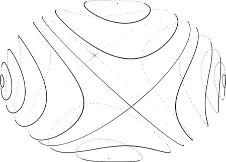
The evolution of the components of the angular momentum on the principal axes has a remarkable property. For almost every initial condition the body components of the angular momentum periodically trace a simple closed curve. Figure 2.3: Trajectories of the components of the angular momentum vector on the principal axes, projected onto a plane. Each closed curve, except for the separatrix, is a different trajectory. All the trajectories shown here have the same energy The above figure shows the components of the angular momentum vector on the principal axes for different initial conditions. For most initial conditions we find a one-dimensional simple closed curve. Some trajectories on the front side appear to cross trajectories on the back side, but this is an artifact of projection. The family of trajectories appears to intersect at two points. The curve that is the union of these trajectories is called a separatrix; it separates different types of motion. The state space for the motion of a rigid body is six-dimensional - the three Euler angles and their time derivatives. Noether’s theorem gives us four conserved quantities - the three components of angular momentum as well as energy. This means the motion only has two degrees of freedom. The numerical result above also shows that the three components of angular momentum trace one-dimensional paths. The total angular momentum is also conserved as its components are conserved. That is, While the components themselves do not change, their projection on to the principal axes change as the axes themselves are in motion, attached to the body. The magnitude of $L$ should be the same even if evaluated in the principal axes coordinates. Therefore, Previously, we found expressions for angular momentum and kinetic energy as: These can be combined to get the following expression for kinetic energy in terms of the components of $L$ Equations 2.59 and 2.60 constrain the motion of the components of angular momentum vector on the principal axes. Eq. 2.59 is the equation of a sphere and Eq. 2.60 is the equation of a triaxial ellipsoid. Since the angular momentum components satisfy both conditions, the component of the $L$ vector moves along the intersection of the angular momentum sphere and the energy ellipsoid. The intersection of a sphere and ellipsoid with the same center typically forms two closed curves. The above equations were constructed with the assumption $A \leq B \leq C$. This means that the longest axis of the ellipsoid corresponds with the $\hat{c}$ direction which is the principal axis with the largest moment of inertia. And similarly the shortest axis of the energy ellipsoid coincides with the $\hat{a}$ direction (prinicipal axis for the smallest moment of inertia). The intersection curves can be seen to shrink to a point for two axes, $\hat{a}$ and $\hat{c}$, corresponding to the principal axes with the largest and smallest moments of inertia, respectively. If the $L$ vector starts at these points, they tend to stay there. This is called an equilibrium point. Small displacements from this point at the start causes them to orbit the equilibrium point. This means that when the body rotates, the principal axes will describe a small orbit around the angular momentum vector in space (since the vector itself is constant). This is called a relative equilibrium. Conversely, for the $\hat{b}$ axis, or the intermediate axis, the curves appear to cross. This is also an equilibrium point. If the angular moment starts exactly at that point, it will stay at that point. However, if the system is slightly displaced, it tends to move away from the point very quickly. This denotes an unstable equilibrium point. So a body starting its rotation close to the intermediate axis will quickly end up in a tumble (while the $L$ vector still remains fixed in space). This leads to the “intermediate axis theorem”, also known as the tennis racket theorem. Now consider the case where the rotating rigid body is somehow dissipating energy - maybe due to some flexing structural member. Since this is an internal process, this only decreases the energy while the angular momentum remains constant. This means that the intersection curve on which the system moves starts to deform. For a given $L$, there is a lower limit for energy. For this lowest energy state, the intersection is a pair of points on the maximum moment of inertia axis. This shows that with dissipating energy, a rotating rigid body ends up rotating around the principal axis of highest inertia - this is the lowest energy state consistent with a constant angular momentum. The deviations from principal axis rotation for the Earth are tiny: the angle between the angular momentum vector and the ĉ axis for the Earth is less than one arc-second. The above-mentioned deviations could be caused by Earthquakes, tides etc. In fact almost every other planet, asteroid and moon rotates about its principal axis with the largest moment of inertia. There are some exceptions - notably comets - which has reactions caused by the volatile jets that affect their rotation as they get closer to the Sun. Among the natural satellites, the only known exception is Saturn’s satellite Hyperion, which is tumbling chaotically. Hyperion is especially out of round and subject to strong gravitational torques from Saturn.2.8.2 Qualitative Features of Free Rigid Body Motion
$$
L^2 = L_x^2 + L_y^2 +L_z^2\tag{2.58}
$$
$$
L^2 = L_a^2 + L_b^2 + L_c^2\tag{2.59}
$$
$$
\begin{align*}
T_R &= \frac{1}{2} \left[ A(\omega^a)^2 + B(\omega^b)^2 + C(\omega^c)^2\right]\tag{2.41}\\
L_a &= A\omega^a\\
L_b &= B\omega^b\\
L_c &= C\omega^c\tag{2.51}\\
\end{align*}
$$
$$
E = \frac{1}{2}\left( \frac{L_a^2}{A} + \frac{L_b^2}{B} + \frac{L_c^2}{C} \right)\tag{2.60}
$$