2.11 Spin Orbit Coupling

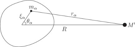
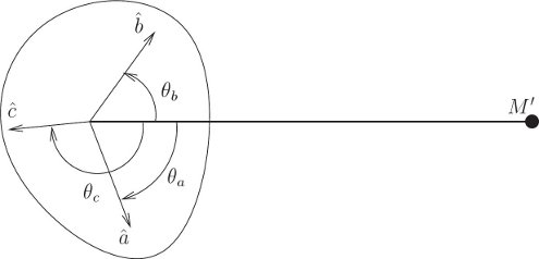
The rotation of planets and natural satellites is affected by the gravitational forces from other celestial bodies. As an extended application of the Lagrangian method for forced rigid bodies, we consider the rotation of celestial objects subject to gravitational forces.

In this section, we will develop expressions for potential energy for the graviational interaction of an “extended body” (i.e. not a point mass) with an external point mass. Combined with the rigid body kinetic energy, this can be used to create Lagrangians that model a number of systems.

2.11.1 Development of the Potential Energy

The rigid body can be modeled as a collection of particles subject to rigid constraints. Similar to the kinetic energy decribed in the previous section, the potential energy of a rigid body can also be expressed in terms of the moment of inertia and later expressed in terms of generalized coordinates.

Figure 2.9 The gravitational potential energy of a point mass and a rigid body is the sum of the gravitational potential energy of the point mass with each constituent mass element of the rigid body.

The gravitational potential energy of a rigid body is the sum of the potential energies of the individual point masses that make up the rigid body.

where $M’$ is the mass of the external point mass that is the source of the gravity, $r_\alpha$ is the distance from the point mass to the component particle in the rigid body and $G$ is the universal gravitational constant. The position of the component particle can be resolved as:

where $\vec{R}$ is the vector from the external point mass to the center of mass of the rigid body. With this formulation, the distance to the particle, $r_\alpha$ becomes, $r_\alpha = R^2 + \xi^2_\alpha - 2R\xi_\alpha \cos\theta_\alpha$, where $\theta_\alpha$ is the angle between the lines from the center of mass to the constituent particle and to the point mass (see Figure 2.9).

Given that this is a three-dimensional body, $\xi_\alpha$ and $\theta_\alpha$ cannot uniquely specify the p0osition of the constituent particle. However, these are the only parameters required to define the potential energy as it is simply a function of the distance between the particle and the distant point mass. The potential energy is therefore defined as:

This can be expanded using Legendre Polynomials. The Legendre polynomials $P_l$ may be obtained by expanding the expression $(1 + y^2 − 2yx)^{1/2}$ as a power series in $y$. The coefficient of $y_l$ is $P_l(x)$. The first few Legendre polynomials are: $P_0(x) = 1$, $P_1(x) = x$, $P_2(x)=\frac{3}{2}x^2−\frac{1}{2}$ , and so on. Then we get the following expression for potential energy:

Successive terms in this expansion typically drop off quickly since the distance between celestial bodies are vastly bigger than their size. Each term in the series has an upper bound. This is because the Legendre polynomials all have a magnitude less than one for arguments between -1 and 1 (which $\cos(\theta_\alpha)$ satisfies), and the distances $\xi_\alpha$ are all less than some maximum size $\xi_{max}$. Therefore, the sum over $m_\alpha$ times the upper bounds of each term is just $M$ times the upper bounds. Therefore,

Successive terms decrease by a factor of $\frac{\xi_{max}}{R}$. A body with a sufficiently strong gravitational force overcomes the material strength of the rigid body and converts it into a sphere over time. The higher order terms in the series are measuring the deviation of the rigid body from a sphere. We can truncate the series to different values of $l$ based on the fidelity required.

When $l=0$, the sum over $\alpha$ gives the total mass $M$ of the rigid body. For $l=1$, the sum is zero because $\vec{\xi}_\alpha$ is defiend relative to the center of mass. For $l=2$, the sum can be written in terms of the moment of inertia of the body as:

where $A, B, C$ are the principal moments of inertia and $I$ is the moment of inertia of the body about the line between the center of mass of the body and the external point mass. $I$ depends on the orientation of the body w.r.t line between the bodies. Therefore, the potential energy of the body with terms up to $l=2$ is:

This is also called MacCullagh’s formula.

Figure 2.10: The orientation of the rigid body is specified by the three angles from the line between the centers and the principal axes.

Figure 2.10 shows a method for computing $I$ in terms of the principal moment of inertia. Let $\theta_a$, $\theta_b$, and $\theta_c$, are the angles of the principal axes $\hat{a}, \hat{b}, \hat{c}$, respectively, from the line connecting the center of mass and the point mass. Then $I$ can be found to be:

The potential energy is then: