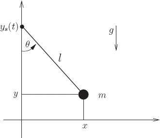
So far we have found $L = T-V$ to be a suitable Lagrangian for systems of point particles subject to forces derived from a potential. In this section, we will find that $L = T − V$, expressed in irredundant coordinates, is also a suitable Lagrangian for modeling systems of point particles with rigid constraints. We start with a system of $N$ point masses, indexed by $\alpha$ in 3D space. We choose a set of generalized coordinates $q$ that have the system constraints built into them. The rectangular coordinates can then be defined as: where all the coordinate constraints are built into the functions $f_\alpha$. The velocities can then be obtained in terms of the generalized velocities, $v$ in the same manner as in the last section as: The kinetic energy in rectangular coordinates can be obtained as: Converting to generalized coordinates: Similarly, the potential energy in generalized coordinates is: The Lagrangian can then be obtained as $L = T - V$. Consider a pendulum of length $l$ and mass $m$, modeled as a point mass, supported by a pivot that is driven in the vertical direction by a given function of time $y_s(t)$. This system has a single degree of freedom and can be represented by the generalized coordinate $\theta$, the angle of the pendulum from the vertical. The position of the bob is given in rectangular coordinates by The velocities are: The kinetic energy is: The potential energy $\widetilde{V}(t; x,y) = mgy$ in rectangular coordinates. Therefore in generalized coordinates,1.6.2 Systems with Rigid Constraints
Lagrangians for rigidly constrained systems
A pendulum driven at the pivot
;; Computing EoMs
(defn T-pend-on-pivot [m l g y_s]
    (fn [[t [theta] [thetadot]]]
        (let [Dy_s ((D y_s) t)]
            (* 1/2 m
               (+ (square (* l thetadot))
                  (square Dy_s)
                  (* 2 l (sin theta) Dy_s thetadot)
              )
           )
        )
    )
)

(defn V-pend-on-pivot [m l g y_s]
    (fn [[t [theta] [thetadot]]]
        (* m g (- (y_s t) (* l (cos theta))))
))

(def L-pend-on-pivot (- T-pend-on-pivot V-pend-on-pivot))

;; (render
;;  (let [local ((Gamma (up (literal-function 'theta))) 't)
;;        L (L-pend-on-pivot 'm 'l 'g (literal-function 'y_s))
;;        ]
;;      (L local)
;;      ))

;; EOMs for pendulum driven at pivot
(let [L (L-pend-on-pivot 'm 'l 'g (literal-function 'y_s))
      state (up (literal-function 'theta))]
   (rendertex (((Lagrange-equations L) state) 't)))
$$
\mathbf{x}_\alpha = f_\alpha(t, q)\\
$$
$$
\mathbf{v}_\alpha = \partial_0 f_\alpha(t, q) + \partial_1 f_\alpha(t, q) v\\
$$
$$
\widetilde{T}(t; x_0 ... x_{N-1}; v_0 ... v_{N-1}) = \sum_\alpha \frac{1}{2} m_\alpha \mathbf{v}_\alpha^2\\
$$
$$
T(t, q, v) = \sum_\alpha \frac{1}{2} m_\alpha \left( \partial_0 f_\alpha(t, q) + \partial_1 f_\alpha(t, q) v \right)
$$
$$
V(t, q, v) = \widetilde{V}(t, f(t, q))
$$
$$
x = l\sin{\theta} \text{ and } y = y_s(t) - l\cos{\theta}
$$
$$
v_x = l\dot{\theta}\cos{\theta} \text{ and } v_y = Dy_s(t) + l\dot{\theta}\sin{\theta}
$$
$$
\begin{align*}
\widetilde{T}(t; x,y; v_x, v_y) &= \frac{1}{2}m(v_x^2 + v_y^2) \\
T(t,\theta,\dot{\theta}) &= \frac{1}{2}m ( (l\dot{\theta}\cos{\theta})^2 + (Dy_s(t) + l\dot{\theta}\sin{\theta})^2 \\
&= \frac{1}{2}m \left( l^2\dot{\theta}^2(\cos^2{\theta} + \sin^2{\theta}) + (Dy_s(t))^2 + 2l\dot{\theta}\sin{\theta}Dy_s(t) \right)\\
&= \frac{1}{2}m \left( l^2\dot{\theta}^2 + (Dy_s(t))^2 + 2l\sin{\theta}Dy_s(t) \dot{\theta} \right)
\end{align*}
$$
$$
V(t,\theta,\dot{\theta}) = mg (y_s(t) - l\cos{\theta})
$$
\begin{bmatrix}\displaystyle{g\,l\,m\,\sin\left(\theta\left(t\right)\right) + {l}^{2}\,m\,{D}^{2}\theta\left(t\right) + l\,m\,\sin\left(\theta\left(t\right)\right)\,{D}^{2}y_s\left(t\right)}\end{bmatrix}