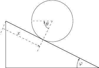
In this section we look at a specific type of velocity-dependent constraints, which are “total-time derivatives” of a velocity independent function. The methods in Section 1.10.1 do not apply here as the constraint is velocity-dependent. Let this constraint $\psi = 0$ be a velocity-dependent constraint. If $\psi$ is a total-time derivative, this means that there exists some velocity-independent function, $\varphi$ such that: Since $\varphi$ is velocity independant, $\partial_2 \varphi = 0$. The relationship between $\psi$ and $\varphi$ can be restated (as local-tuple functions) as: We can find $\psi$ by solving this PDE. The constraint is defined as $\psi = 0$. This implies that $\varphi = K$ for some constant $K$. Conversely, if we know that $\varphi = K$, then $\psi = 0$ follows. Thus, the velocity-dependent constraint, $\psi = 0$ is equivalent to the velocity-independent constraint, $\varphi = K$. If $L$ is the unconstrained Lagrangian, the Lagrange equations with the constraint $\varphi = K$ are: where $\lambda$ is a function of time that will be eliminated during the solution process. $K$ can be ignored here as $\lambda(\varphi - K)$ and $\lambda(\varphi)$ result in the same Lagrange equations. The function $\varphi$ is independent of velocity and $\partial_2 \varphi = 0$. So we can use the same techniques from Section 1.10.1 to get the Lagrange equations for the system as: From Eq. 1.214, we can also infer that $\psi$ is the partial of $\varphi$ w.r.t velocity, or $\partial_2 \psi = \partial_1 \varphi$. Therefore, the Lagrange equations with the constraint $\psi = 0$ can also be written as: This is important because it shows that we can write the Lagrangian in terms of $\psi$ without having to compute $\varphi$, as long as we can show that $\varphi$ exists. We can also get the same result using the Augmetned Lagrangian technique. Consider the augmented Lagrangian below The Lagrange equations for $L’$ are: where $D\lambda’ = \lambda$. This shows that Eq. 1.218 and Eq. 1.219 are the same equations. The technique defined in this section can be used for systems with constraints that can be written in terms of the derivative of a velocity-independent constraint. Such constraints are called integrable constraints. Any system where the constraints are coordinate constraints, or can be put in the form of a coordinate constraint are called holonomic constraints. $$\require{cancel}$$ Figure 1.10: A massive hoop rolling, without slipping, down an inclined plane. “Goldstein’s hoop” is an example of a dynamic system with an integrable constraint: a hoop of mass $M$ and radius $R$ rolling down a one-dimensional inclined plane (Figure 1.10). This problem can be formulated in terms of two coordinates, $\varphi$, the angular displacement of an arbitrary point on the hoop from some arbitrary reference line, and $x$, the linear progress of the center of the hoop down the plane. The cojnstraint is that the hoop rolls without slipping, or in other words, the change is $\theta$ is directly reflected a change in $x$. The constraint function is: This constraint is represented as a relation between generalized velocities, which can be integrated to get $x = R\theta + c$. This integrated constraint is a velocity-independent constraint. The augmented Lagrangian can be formulated in terms of the original constraint or its derivative. The kinetic energy consists of the energy of rotation of the hoop (described later in Chapter 2 as $\frac{1}{2}MR^2\dot{\theta}^2$) and the energy from the motion of its center of mass. The potential energy of the system decreses as the hoop proceeds down the slope. Thus the augmented Lagrangian is: Lagrange equations for this Lagrangian can be obtained as: Differentiating the third equation, we get Multiplying Eq. 1.223 by R and adding with Rq. 1.224 This acceleration is just half of what the acceleration would have been for a point mass sliding down a frictionless inclied plane. Also notable is that the acceleration is independent of both $M$ and $R$. From the Lagrange equations, $D\lambda$ can be interepreted as the frictional force that is causing the hoop to roll instead of slide. Combining Eq. 1.223 and Eq. 1.227, this force can be found to be: and the angular acceleration $D^2\theta$ is:1.10.2 Derivative Constraints
Goldstein’s Hoop
$$
\psi \circ \Gamma[q] = D(\varphi \circ \Gamma[q])
$$
$$
\psi = D_t \varphi = \partial_0 \varphi + \partial_1 \varphi \dot{Q}\tag{1.214}
$$
$$
\mathscr{E}[L] \circ \Gamma[q] + \lambda(\mathscr{E}[\varphi] \circ \Gamma[q]) = 0\\
$$
$$
\mathscr{E}[L] \circ \Gamma[q] - \lambda(\partial_1 \varphi \circ \Gamma[q]) = 0\\
$$
$$
\mathscr{E}[L] \circ \Gamma[q] - \lambda(\partial_2 \psi \circ \Gamma[q]) = 0\tag{1.218}
$$
$$
L' = L + \lambda' \psi\\
$$
$$
\mathscr{E}[L'] \circ \Gamma[q] = -D\lambda (\partial_2 \varphi \circ \Gamma[q]) \tag{1.218}
$$
$$
\psi(t; x,\theta; \dot{x},\dot{\varphi}) = R\dot{\theta} - \dot{x} = 0\\
$$
$$
L(t; x,\theta,\lambda; \dot{x},\dot{\theta},\dot{\lambda}) = \frac{1}{2}MR^2\dot{\theta}^2 + \frac{1}{2}M\dot{x}^2 - (-Mg x\sin\varphi) + \lambda(R\dot{\theta} - \dot{x})\tag{1.122}
$$
$$
\begin{align*}
M D^2x - D\lambda &= Mg \sin\varphi \tag{1.223}\\
M R^2 D^2\theta + R D\lambda &= 0 \tag{1.224}\\
R D\theta - Dx &= 0 \tag{1.225}\\
\end{align*}
$$
$$
R D^2\theta = D^2 x\tag{1.226}
$$
$$
\begin{align*}
0 &= M R D^2x - \cancel{RD\lambda} - M R g \sin\varphi
+ M R^2 D^2\theta + \cancel{R D\lambda} \\
&= \cancel{M} \cancel{R} D^2x - \cancel{M} \cancel{R} g \sin\varphi + \cancel{M} R^\cancel{2} D^2\theta \\
&= D^2x + R D^2\theta - g \sin\varphi \\
&= 2 D^2x - g\sin\varphi \\
=> D^2x &= -\frac{1}{2}g\sin\varphi \tag{1.227}
\end{align*}
$$
$$
D\lambda = \frac{1}{2} Mg \sin\varphi\tag{1.228}
$$
$$
-\frac{1}{2}\frac{g}{R}\sin\varphi\tag{1.229}
$$