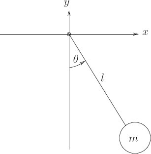
In the previous section, we showed that for motion of a system with the constraint $\varphi(t, q(t), Dq(t)) = 0$, for stationary action, the path variations, $\eta(t)$, must be tangent to the constraint surface. And in order for the variation to be tangent to the constraint at a given time, it must satisfy the condition: Now consider constraints that are only functions of the coordinates, i.e, Now the variation is tangent to the constraint if We also know from Eq. 1.183 in the previous section that, Eq. 1.186 and 1.183 together should determine the motion of the constrained system. Eq 1.183 is satisfied if the dot product of the first term (aka the residual of Lagranges Equations) and $\eta(t)$ is zero at all times. This is also the definition for two functions of time to be orthogonal to each other. To quote footnote 92 from the book: We take two tuple-valued functions of time to be orthogonal if at each instant the dot product of the tuples is zero. Similarly, tuple-valued functions are considered parallel if at each moment one of the tuples is a scalar multiple of the other. The scalar multiplier is in general a function of time. So the residual of the Lagrange equations is orthogonal to any $\eta(t)$. Also, $\eta(t)$ is tangent to the constraint surface, which means that it is orthogonal to the normal to the constraint surface. A vector that is orthogonal to all vectors orthogonal to a given vector is parallel to the given vector. Therefore, the residual of Lagrange equations is parallel to the normal to the constraint surface; which means the two functions are proportional: The proportionality factor $\lambda$ is itself a function of time and need not be a constant. This equation, along with the constraint equation $\varphi \circ \Gamma[q] = 0$ is enough to determine the path $q$ and to eliminate the unknown function $\lambda$. We can now form an augmented Lagrangian by treating $\lambda$ as one of the coordinates. The Lagrange equations associated with the coordinates are just the modified Lagrangian in Eq. 1.187. The equation assoicated with $\lambda$ is just the constraint equation. So the system is fully specified. This Lagrangian is also of the same form as the one described in Section 1.6.2. If the new function $\lambda$, can be written as a composition of a local tuple function over the original, unaugmented path: $\lambda = \Lambda \circ \Gamma[q]$, then it is a redundant degree of freedom and can be eliminated from the system if required. Consider the Lagrangian with an extra term $\Lambda\varphi$ where $\varphi$ is the constraint function: The Lagrange equations for $L’‘$ is the same as that for $L$ but with some extra terms arising from $\Lambda\varphi$. Applying the Euler-Lagrange operator to $L’’$: Composing $\mathscr{E}[L]$ with $\Lambda[q]$ results in the Lagrange equations for $L’’$. Since the constraints are satisfied on the path, $\varphi \circ \Gamma[q] = 0$, which implies that $D_t(\Lambda \circ \Gamma[q]) = 0$. Therefore, composing $\mathscr{E}[L]$ with $\Lambda[q]$, we get: $\partial_2\varphi = 0$ as the constraints do not depend on velocity. Then, We can see here that the Lagrange equations for $L’‘$ is the same as that for $L’$, with an extra term. Comparing this to Eq. 1.187, we can see that $\lambda = \Lambda \circ \Gamma[q]$, which is determined purely by the unaugmented state. Therefore $\lambda$ can be eliminated from the Lagrange equations of the augmented Lagrangian. The explicit Lagrange equations derived from the augmented Lagrangian depend on the accelerations $D^2 q$ as well as $\lambda$. Now that $\lambda$ has been showed to be derived purely form the unaugmented state, so too is $D^2 q$ (as there are no other elements in the dynamic equations). Therefore the dynamic evolution of the system is determined purely by the dynamical state. $$\require{cancel}$$ Figure 1.8 The pendulum can be modeled as a point-mass constrained to always be at a constant distance from a pivot point. The system can be represented by the following Lagrangian and constraint: The augmented Lagrangian is: The Lagrange equations for this augmented Lagrangian is: These equations can be simplified by switching to polar coordinates, $x = r\sin{\theta}$ and $y = -r\cos{\theta}$. Substituting this in the constraint equation, we get, $r = l$. Plugging this into the equations 1.196 and 1.197: Multiply Eq. 1.200 by $\cos\theta$ and Eq. 1.201 by $\sin{\theta}$ and add to get: This is indeed the same equation as what we get if we used $\theta$ as an unconstrained generalized coordinate for the pendulum. We can also compute $\lambda$ in terms of the other variables from Eq.1.196 as: This further confirms what we showed in the previous section, that $\lambda$ really is the composition function of the local state of the path. Also, to be noted here is the $2l\lambda$ is a force – the sum of the outward component of gravity and the centrifugal force. This is the tension in the pendulum rod. It is effectively the force that is constraining the mass to stay at a constant distance from the pivot. Figure 1.9: A compound spring-mass system is decomposed into two subsystems. We can analyze compound systems using augmented Lagrangians to enforce constraints between the individual parts. Consider the compound spring-mass system at the top of Figure 1.9. One way to analyze this is as a single system with two coordinates $x_1$ and $x_2$ to represent the extension of the springs from their equilibrium lengths of $X_1$ and $X_2$. An alternative procedure would be to break it into two parts – one being the spring-mass attached to the wall, and the other being the second spring-mass system with its attachment point specified by an additional coordinate $\xi$ (which may have its own velocity). The Lagrangian for each part can be written separately. The Lagrangian of the combined system is the sum of the two component Lagrangians along with a constraint $\xi = X_1 + x_1$ to ensure that the two systems are attached. So the Lagrangian for the part attached to the wall is: and the Lagrangian for the part that attaches to it is: Combining the two Lagrangians with the contact constraint, we get: The Lagrange’s equations for the system are: For eliminating $\xi$ and $\lambda$, substitute Eq. 1.210 into Eq. 1.209, Substituting for $\lambda$ in Eq. 1.207, Substituting for $\xi$ in Eq. 1.208, Equations 1.211 and 1.212 are the equations of motion for the compound system. This is a general strategy that can be used to create a library of primitive components. Each component may be characterized by a Lagrangian with additional degrees of freedom for the terminals where that component may be attached to others. We then can construct composite Lagrangians by combining components, using constraints to glue together the terminals.1.10.1 Coordinate Constraints
How do we eliminate $\lambda$ from the Lagrange Equations?
The Pendulum using Constraints
Building systems from parts
$$
\begin{align*}
(\partial_1 \varphi \circ \Gamma[q])\eta + (\partial_2 \varphi \circ \Gamma[q])D\eta = 0
\end{align*}
$$
$$
\partial_2 \varphi = 0\\
$$
$$
(\partial_1 \varphi \circ \Gamma[q])\eta = 0 \tag{1.186}
$$
$$
\{ (\partial_1 L \circ \Gamma[q]) - D\left( \partial_2 L \circ \Gamma[q] \right) \} \eta = 0 \tag{1.183}
$$
$$
(\partial_1 L \circ \Gamma[q]) - D\left( \partial_2 L \circ \Gamma[q] \right) = \lambda (\partial_1 \varphi \circ \Gamma[q])\tag{1.187}
$$
$$
L'(t; q,\lambda;\dot{q},\dot{\lambda}) = L(t,q,\dot{q})+ \lambda\varphi(t,q,\dot{q})
$$
$$
L'' = L + \Lambda\varphi\\
$$
$$
\begin{align*}
\mathscr{E}[L''] &= \mathscr{E}[L + \Lambda\varphi] = \mathscr{E}[L] + \mathscr{E}[\Lambda\varphi]\\
&= \mathscr{E}[L] + \mathscr{E}[\Lambda] \varphi + \Lambda\mathscr{E}[\varphi] + (D_t \Lambda)\partial_2 \varphi + (D_t \varphi)\partial_2 \Lambda
\end{align*}
$$
$$
\begin{align*}
\mathscr{E}[L'']\circ\Gamma[q] &= \mathscr{E}[L]\circ\Gamma[q] + (\mathscr{E}[\Lambda]\circ\Gamma[q])\underbrace{\cancel{\varphi}}_{=0}
+ \underbrace{(\Lambda\circ\Gamma[q])}_{=\lambda}(\mathscr{E}[\varphi]\circ\Gamma[q])\\
&\quad+ (D_t \Lambda)(\partial_2 \varphi\circ\Gamma[q]) + (\underbrace{\cancel{D_t \varphi}}_{=0})(\partial_2 \Lambda\circ\Gamma[q]) \\
&= \mathscr{E}[L]\circ\Gamma[q] + \lambda(\mathscr{E}[\varphi]\circ\Gamma[q]) + (D_t \Lambda)(\partial_2 \varphi\circ\Gamma[q])
\end{align*}
$$
$$
\mathscr{E}[L'']\circ\Gamma[q] = \mathscr{E}[L]\circ\Gamma[q] + \lambda(\mathscr{E}[\varphi]\circ\Gamma[q])\tag{1.192}
$$
$$
\begin{align*}
L(t; x,y; v_x,v_y) &= \frac{1}{2} m (v_x^2 + v_y^2) - mgy\\
x^2+y^2-l^2 &= 0
\end{align*}
$$
$$
L(t; x,y,\lambda; v_x,v_y,\dot{\lambda}) = \frac{1}{2} m (v_x^2 + v_y^2) - mgy + \lambda(x^2+y^2-l^2)\\
$$
$$
\begin{align*}
m D^2x - 2\lambda x = 0 \tag{1.196}\\
m D^2y + mg - 2\lambda y = 0 \tag{1.197}\\
x^2 + y^2 - l^2 = 0\tag{1.198}\\
\end{align*}
$$
$$
\begin{align*}
0 & = m D^2 (l\sin\theta) - 2\lambda l\sin\theta \\
& = m (D(l \cos\theta D\theta)) - 2\lambda l\sin\theta\\
0 &= ml (\cos\theta D^2\theta - \sin\theta (D\theta)^2) - 2\lambda l\sin\theta \tag{1.200}
\end{align*}
$$
$$
\begin{align*}
0 &= m D^2 (-l\cos\theta) + mgl - 2\lambda (-l\cos\theta) \\
&= m (D(l \sin\theta D\theta)) + 2\lambda l\cos\theta \\
0 &= ml (\sin\theta D^2\theta + \cos\theta (D\theta)^2) + 2\lambda l\cos\theta + mg \tag{1.201}
\end{align*}
$$
$$
\begin{align*}
0 &=ml (\cos\theta D^2\theta - \sin\theta (D\theta)^2)\cos\theta - \cancel{2\lambda l\sin\theta \cos \theta}\\
& \quad+ ml (\sin\theta D^2\theta + \cos\theta (D\theta)^2)\sin\theta + \cancel{2\lambda l\cos\theta \sin\theta} + mg\sin\theta\\
&= ml (\cos^2\theta D^2\theta) - \cancel{ml \sin\theta \cos\theta(D\theta)^2} \\
& \quad+ ml (\sin^2 \theta D^2\theta) + \cancel{ml \cos\theta \sin\theta(D\theta)^2} + mg\sin\theta \\
&=ml D^2\theta (\cos^2\theta + \sin^2 \theta ) + mg\sin\theta \\
0&= ml D^2\theta + mg\sin\theta
\end{align*}
$$
$$
\begin{align*}
\lambda &= \frac{m D^2 x}{2x} = \frac{m D^2 (l\sin\theta)}{2l\sin\theta} \\
&= \frac{m (D(l \cos\theta D\theta))}{2l\sin\theta} \\
&= \frac{ml \cos\theta D^2\theta - ml \sin\theta (D\theta)^2}{2l\sin\theta} \\
&= \frac{\overbrace{ml D^2\theta}^{-mg\sin\theta}\cos\theta - ml \sin\theta (D\theta)^2}{2l\sin\theta} \\
&= \frac{-mg\cancel{\sin\theta}\cos\theta - ml \cancel{\sin\theta} (D\theta)^2}{2l\cancel{\sin\theta}} \\
\lambda & = \frac{-1}{2l} \left(mg\cos\theta - ml(D\theta)^2\right)
\end{align*}
$$
$$
L_1(t; x_1; \dot{x_1}) = \frac{1}{2}m_1\dot{x_1}^2 - \frac{1}{2}k_1 x_1^2\\
$$
$$
L_2(t; \xi,x_2; \dot{\xi},\dot{x_2}) = \frac{1}{2}m_2(\dot{\xi} + \dot{x_2})^2 - \frac{1}{2}k_2 x_2^2\\
$$
$$
L(t; x_1, x_2, \xi; \dot{x_1},\dot{x_2},\dot{\xi}) = L_1(t; x_1; \dot{x_1}) + L_2(t; \xi,x_2; \dot{\xi},\dot{x_2}) + \lambda(\xi - (X_1 + x_1))
$$
$$
\begin{align*}
m_1D^2 x_1 = -k_1 x_1 - \lambda \tag{1.207} \\
m_2(D^2\xi + D^2 x_2) = -k_2 x_2 \tag{1.208} \\
m_2(D^2\xi + D^2 x_2) = \lambda \tag{1.209} \\
0 = \xi - (X_1 + x_1) \tag{1.210}
\end{align*}
$$
$$
m( \underbrace{D^2X_1}_{=0} + D^2 x_1 + D^2 x_2 ) = \lambda\\
$$
$$
\begin{align*}
m_1 D^2 x_1 &= -k_1 x_1 - m_2 D^2 x_1 - m_2 D^2 x_2\\
m_1 D^2 x_1 + m_2 (D^2 x_1 + D^2 x_2) + k_1 x_1 &= 0\tag{1.211}
\end{align*}
$$
$$
\begin{align*}
m_2(D^2 x_1+ D^2 x_2) + k_2 x_2 &= 0\tag{1.212}
\end{align*}
$$