Deriving the MSL/Apollo Entry Guidance Algorithm

This post is a companion to the video linked above and includes a full derivation of the Apollo entry guidance longitudinal control algorithm. Please watch the video for more context. Full source code of Jupyter notebooks implementing the algorithm can be found at thomasantony/msl-apollo-entry-guidance.

NASA’s Mars Science Laboratory mission showcased an advancement in entry technology that allowed it to land much closer to its designated landing site than previous missions. It used with great success, the same guidance algorithm originally used by the Apollo Command Module when returning from the moon. By modulating its lift vector, MSL was able to counteract errors in its trajectory during hypersonic flight and combined with the famous “sky-crane” maneuver, deliver the Curiosity rover to within 2.5 km of its targeted landing site next to Gale Crater. Last year’s Mars 2020 mission used the same guidance system to successfully land the Perseverance rover within Jezero crater.

Apollo Guidance Algorithm Overview

The goal of the Apollo guidance algorithm is to minimize the error in “range” along the ground when compared to that of a pre-computed reference trajectory. It does not try to exactly match the reference trajectory, but instead computes a constant bank angle that is supposed to minimize the downrange distance error at the point where the vehicle reaches terminal altitude. This computation is repeated several times a second in the same manner as a closed-loop control system to correct for deviations in the trajectory due to external or internal factors.

The guidance algorithm uses bank angle to control the amount of vertical lift. This has the side-effect of causing lateral motion that takes the spacecraft away from the desired path. In order to account for this, the bank angle commanded is reversed when the predicted cross-range error exceeds a certain amount, effectively creating a series of S-turns. This is similar to the S-turns performed by the Space Shuttle during its re-entry.

This article focuses on the downrange error control.

2DOF Dynamic Model

The MSL entry vehicle is modeled in two-dimensions using a vehicle-centric polar coordinate system. The state variables in the model are altidude ($h$), downrange distance ($s$), speed ($v$) and flight path angle($\gamma$). Their equations of motion are as follows:

$$ \begin{align*} \frac{d h}{dt} &= v \sin{\gamma} \nonumber \\ \frac{d s}{dt} &= v \cos{\gamma} \\ \frac{d v}{dt} &= -{{D/m}} - {{g}} \sin(\gamma) \\ \frac{d \gamma}{dt} &= \frac{1}{v} \left(\frac{v^2 \cos(\gamma)}{{{R_M}} + h} + \frac{L \cos{u}}{m} - {{g}}\cos(\gamma)\right) \\ \end{align*} $$

where

$$ \begin{align*} \frac{D}{m} &= \frac{\rho v^2}{2 \beta} &;& \text{ Drag Acceleration}\\ \frac{L}{m} &= \frac{D}{m}\enspace (L/D) &;&\text{ Lift Acceleration}\\ \nonumber\\ \rho &= \rho_0 e^{-h/H} &;& \text{ Atmosphere Model}\\ \nonumber\\ \beta &= 120 \text{kg/m$^2$} &;& \text{ Ballistic Coefficient} \\ (L/D) &= 0.24 &;&\text{ Lift-to-Drag Ratio} \end{align*} $$

Surface atmospheric density, $\rho_0$ and scale height, $H$ define the exponential atmospheric model. $g$ is a constant value for acceleration due to gravity. $u$ is the bank angle of the vehicle. The states are collectively referred to as $\mathbf{x}$. The equations of motions may be collectively referred to as $\mathbf{f}(\mathbf{x}, u, t)$.

Deriving the Apollo Entry Guidance Algorithm

Note on the Variation Operator

This derivation requires the use of the “variation operator”, denoted by $\delta$, sometimes called a functional derivative or variational derivative. A functional is a function that acts on functions. For example, $J(y(t))$ is a functional because $y$ is itself a function of time. Here $J$ is a scalar quantity derived from a function $y(t)$, that essentially consists of an infinite number of points.

The variational operator is to functionals, what derivatives are to functions. Similar to how a stationary point of a function can be found by setting its derivative to zero, the stationary point of a functional can be found by setting its variation to zero.

Please check the following links if you want to learn more:

https://www.youtube.com/watch?v=vqDHO2eKXcs

https://canvas.vt.edu/files/1315932/download?download_frd=1

Deriving bank angle policy

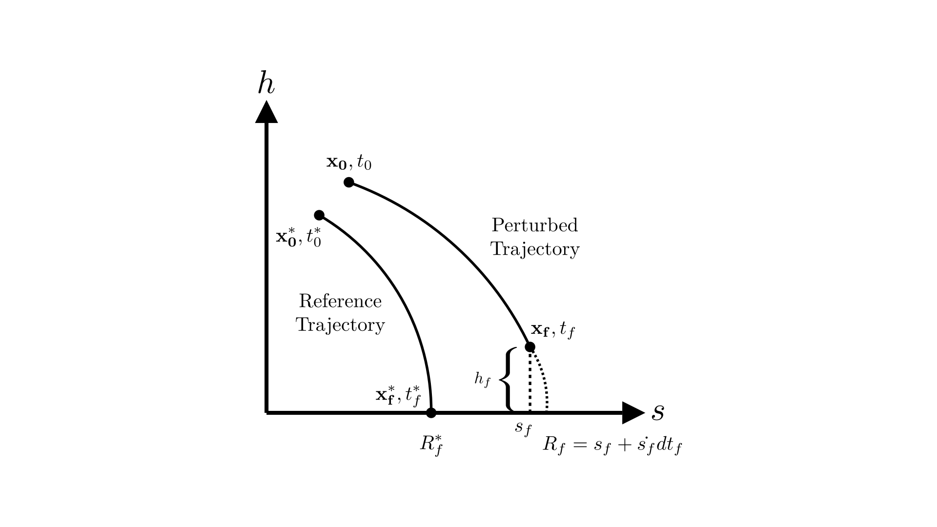
Reference Trajectory and Perturbed Trajectory

The goal is to find the constant bank angle $u$ that will guide the spacecraft from the perturbed starting state $\mathbf{x_0}$ to the same range as the reference trajectory. Let’s call this function $J$. Any variable with an “f” in the suffix denotes that it is evaluated at the terminal point of the trajectory and the ‘*’ denotes that it is part of the reference trajectory.

$$ \begin{align} J = R_f &= s_f + \dot{s_f} dt_f = s_f + v_f \cos(\gamma_f) dt_f \label{eqn:J_1} \end{align} $$

From the equations of motion,

$$ \begin{align} \dot{h_f} &= \frac{dh_f}{dt_f} \implies dt_f = \frac{dh_f}{\dot{h_f}} \label{eqn:h_f_expr} \end{align} $$

Substituting $\eqref{eqn:h_f_expr}$ in $\eqref{eqn:J_1}$,

$$ \begin{align} J &= s_f + \frac{v_f \cos(\gamma_f) }{\dot{h_f}} dh_f \\ &= s_f + \frac{v_f \cos(\gamma_f)}{v_f \sin(\gamma_f)} dh_f \end{align} $$

Assuming that the reference trajectory terminates at the ground, we get $dh_f = 0 - h_f = -h_f$

$$ \implies J = s_f - cot(\gamma_f) h_f = \Phi(\mathbf{x}_f) $$

We want to now find a constant value of $u$ that will keep J constant at $J = R_f = R_f^*$ even with perturbations. We are able to control the trajectory by influencing $u$ and are constrained by physics i.e. equations of motion, $\dot{\mathbf{x}} = \mathbf{f}(\mathbf{x},u,t)$. These constraints can be adjoined to $J$ using co-states $\mathbf{\lambda}^\intercal = \left[\lambda_h\enspace\lambda_s\enspace\lambda_v\enspace\lambda_\gamma\right]$, one for each state. This is very similar to Lagrange multipliers used in function optimization. In this case, each costate is a function that has its own equation of motion which will be derived here.

$$ J' = \Phi(\mathbf{x}_f) + \int_{t_0}^{t_f} \mathbf{\lambda}^\intercal(t) \left\{ \mathbf{f}(\mathbf{x},u, t) - \dot{\mathbf{x}}\right\} dt $$

To find the stationary point of $J$ we apply the variation operator. We also shorten $\mathbf{f}(\mathbf{x},u, t)$ to just $\mathbf{f}$.

$$ \begin{align} \delta J' &= \frac{\partial \Phi}{\partial \mathbf{x}}\delta \mathbf{x}\bigg|_{t=t_f} + \delta \left[ \int_{t_0}^{t_f} \mathbf{\lambda}^\intercal(t) \left\{ \mathbf{f} - \dot{\mathbf{x}}) \right\} dt \right] \nonumber\\ &= \frac{\partial \Phi}{\partial \mathbf{x}}\delta \mathbf{x}\bigg|_{t=t_f} + \delta \int_{t_0}^{t_f} \bigg[ \mathbf{\lambda}^\intercal(t) \mathbf{f} - \mathbf{\lambda}^\intercal(t)\dot{\mathbf{x}}\bigg] dt \nonumber\\ &= \frac{\partial \Phi}{\partial \mathbf{x}}\delta \mathbf{x}\bigg|_{t=t_f} + \int_{t_0}^{t_f} \delta \big[ \mathbf{\lambda}^\intercal(t) \mathbf{f} \big] - \delta\big[\mathbf{\lambda}^\intercal(t)\dot{\mathbf{x}}\big] dt \nonumber\\ &= \frac{\partial \Phi}{\partial \mathbf{x}}\delta \mathbf{x}\bigg|_{t=t_f} + \int_{t_0}^{t_f} \delta \big[ \mathbf{\lambda}^\intercal(t) \mathbf{f} \big] - \delta\big[\mathbf{\lambda}^\intercal\dot{\mathbf{x}}\big] dt \end{align} $$

Applying the chain rule to the variation operator

$$ \begin{align} \delta J' &= \frac{\partial \Phi}{\partial \mathbf{x}}\delta \mathbf{x}\bigg|_{t=t_f} + \int_{t_0}^{t_f} \mathbf{\lambda}^\intercal \delta \mathbf{f} + \delta\mathbf{\lambda}^\intercal \mathbf{f} - \delta\mathbf{\lambda}^\intercal(t)\dot{\mathbf{x}} - \mathbf{\lambda}^\intercal\delta\dot{\mathbf{x}} \enspace\enspace dt \label{eqn:Jprime_1} \end{align} $$

Applying Leibniz Rule to the first term of the integral in ${\eqref{eqn:Jprime_1}}$,

$$ \begin{align} \int_{t_0}^{t_f} \mathbf{\lambda}^\intercal \delta \mathbf{f}(\mathbf{x}, u, t)\enspace dt = \int_{t_0}^{t_f} \mathbf{\lambda^\intercal} \frac{\partial \mathbf{f}}{\partial \mathbf{x}} \delta\mathbf{x} + \mathbf{\lambda^\intercal} \frac{\partial \mathbf{f}}{\partial \mathbf{u}} \delta\mathbf{u}\enspace dt \label{eqn:Jprime_int_term1} \end{align} $$

Integrating by parts, the fourth term of the integral in ${\eqref{eqn:Jprime_1}}$,

$$ \begin{align} \int_{t_0}^{t_f} \mathbf{\lambda}^\intercal(t)\enspace\delta\dot{\mathbf{x}}\enspace dt &= \int_{t_0}^{t_f} \frac{d}{dt}\big( \mathbf{\lambda}^\intercal \delta \mathbf{x} \big) dt - \int_{t_0}^{t_f} \dot{\mathbf{\lambda}}(t)\enspace\delta x \enspace dt \\ &= \bigg[ {\lambda}^\intercal \delta \mathbf{x} \bigg]_{t_0}^{t_f} - \int_{t_0}^{t_f} \dot{\mathbf{\lambda}}(t)\enspace\delta x \enspace dt \label{eqn:Jprime_int_term4} \end{align} $$

Substituting $\eqref{eqn:Jprime_int_term1}$ and $\eqref{eqn:Jprime_int_term4}$ in ${\eqref{eqn:Jprime_1}}$,

$$ \begin{align} \delta J' &= \frac{\partial \Phi}{\partial \mathbf{x}}\delta \mathbf{x}\bigg|_{t=t_f} + \int_{t_0}^{t_f} \mathbf{\lambda^\intercal} \frac{\partial \mathbf{f}}{\partial \mathbf{x}} \delta\mathbf{x} + \mathbf{\lambda^\intercal} \frac{\partial \mathbf{f}}{\partial \mathbf{u}} \delta\mathbf{u} + \delta\mathbf{\lambda}^\intercal \overbrace{\left(\mathbf{f} - \dot{\mathbf{x}}\right)}^{= 0} \enspace dt - \bigg[ {\lambda}^\intercal \delta \mathbf{x} \bigg]_{t_0}^{t_f} + \int_{t_0}^{t_f} \dot{\mathbf{\lambda}}(t)\enspace\delta x \enspace dt \\ \delta J' &= \bigg[\bigg(\frac{\partial \Phi}{\partial \mathbf{x}} - \mathbf{\lambda}^\intercal\bigg)\delta \mathbf{x}\bigg]_{t=t_f} + \left( \mathbf{\lambda}^\intercal \delta \mathbf{x} \right)\bigg|_{t=t_0}+ \int_{t_0}^{t_f} \delta\mathbf{x}(\mathbf{\lambda}^\intercal\frac{\partial \mathbf{f}}{\partial \mathbf{x}} + \dot{\mathbf{\lambda}}) \enspace dt + \int_{t_0}^{t_f} \mathbf{\lambda}^\intercal \frac{\partial \mathbf{f}}{\partial \mathbf{u}} \delta\mathbf{u} \enspace dt\label{eqn:Jprime_2} \end{align} $$

Set $\delta J’ = 0$ to find the stationary point of $J’$. We choose co-states to have the following equations of motion so that they cancel out the third term in $\eqref{eqn:Jprime_2}$:

$$ \begin{align} \mathbf{\dot{\lambda}} = -\mathbf{\lambda}^\intercal\frac{\partial \mathbf{f}}{\partial \mathbf{x}} \label{eqn:costate_eom} \end{align} $$

Now focusing on the first term of $\eqref{eqn:Jprime_2}$,

$$ \begin{align} \text{Let }\bigg[\bigg(\frac{\partial \Phi}{\partial \mathbf{x}} - \mathbf{\lambda}^\intercal\bigg)\delta \mathbf{x}\bigg]_{t=t_f} &= 0 \nonumber \\ \implies \mathbf{\lambda}^\intercal(t_f) &= \frac{\partial \Phi(t_f)}{\partial \mathbf{x}(t_f)} \label{eqn:costate_bc_vec} \end{align} $$

This gives us the boundary conditions on the costates as follows:

$$ \begin{align} \lambda_h(t_f) &= \frac{\partial \Phi}{\partial h_f} = - \cot{\gamma_f} \\ \lambda_s(t_f) &= \frac{\partial \Phi}{\partial s_f} = 1 \\ \lambda_v(v_f) &= \frac{\partial \Phi}{\partial v_f} = 0 \\ \lambda_\gamma(t_f) &= \frac{\partial \Phi}{\partial \gamma_f} = 0 \\ \end{align} $$

Therefore, assuming the conditions in $\eqref{eqn:costate_eom}$ and $\eqref{eqn:costate_bc_vec}$ hold for the costates, the condition for the stationary point of $J’$ is given by:

$$ \delta J' = \mathbf{\lambda}^\intercal(t_0) \delta \mathbf{x}(t_0) + \int_{t_0}^{t_f} \mathbf{\lambda^\intercal}\frac{\partial \mathbf{f}}{\partial \mathbf{u}} \delta u\enspace dt = 0\\ $$

Apollo guidance assumes that the bank angle correction, $\delta u$ is constant for the whole trajectory.

$$ \begin{align} \mathbf{\lambda}^\intercal(t_0) \delta \mathbf{x}(t_0) &= - \delta u \int_{t_0}^{t_f} \mathbf{\lambda^\intercal}\frac{\partial \mathbf{f}}{\partial \mathbf{u}}\enspace dt \\ \delta u &= -\frac{\mathbf{\lambda}^\intercal(t_0) \delta \mathbf{x}(t_0)}{\int_{t_0}^{t_f} \mathbf{\lambda^\intercal}\frac{\partial \mathbf{f}}{\partial \mathbf{u}}\enspace dt} \label{eqn:delu_1} \end{align} $$

Eq. $\eqref{eqn:delu_1}$ is giving us a “correction factor” for the bank angle $u$ that should minimize the range error at the terminal point if applied over the entire trajectory. This needs to be simplified into something that can be computed on-board the flight computers.

Looking at just the numerator of $\eqref{eqn:delu_1}$.

$$ \mathbf{\lambda}^\intercal(t_0) \delta\mathbf{x}(t_0) = \lambda_h(t_0) \delta h(t_0) + \lambda_s(t_0) \delta s(t_0) + \lambda_v(t_0) \delta v(t_0) + \lambda_\gamma(t_0) \delta \gamma(t_0) $$

Since we are trying to keep $J$ stationary about the reference trajectory, all of the terms here must be evaluated w.r.t the reference trajectory (denoted by the $^*$). We also change the independent variable to the velocity, $v$ as that is a better value for matching up the current state of the vehicle to the reference state (for computing the $\delta$’s).

$$ \begin{align} \mathbf{\lambda^*}^\intercal(v_0) \delta\mathbf{x}(v_0) = \lambda_h^*(v_0) \delta h(v_0) + \lambda_s^*(v_0) \delta s(v_0) + \lambda_v^*(v_0) \underbrace{\delta v(v_0)}_{ = 0} + \lambda_\gamma^*(v_0) \delta \gamma(v_0) \label{eqn:delu_numerator} \end{align} $$

Also, the altitude rate $\dot{h}$ and drag acceleration $D/m$ are more accurately estimated by sensors on board the spacecraft than the altitude or flight-path angle.

$$ \begin{align} \dot{h} &= v \sin{\gamma} \nonumber\\ \implies \delta \dot{h} &= \sin{\gamma} \overbrace{\delta v}^{=0} + v \cos{\gamma} \delta \gamma \nonumber\\ \implies \delta \dot{\gamma} &= \frac{\delta\dot{h}}{v \cos{\gamma}} \label{eqn:delgam_to_delhdot}\\ \end{align} $$

Assuming exponential atmospheric model with scale height $H$,

$$ \begin{align} \frac{D}{m} &= \frac{\rho_0 e^{-h/H} v^2 C_d A_{ref}}{2m}\nonumber\\ \delta(\frac{D}{m}) &= \frac{\rho_0 e^{-h/H} C_d A_{ref}}{2m} (v^2 \frac{\delta h}{H} + 2v\overbrace{\delta v}^{=0})\nonumber\\ \implies \delta(\frac{D}{m}) &= -\frac{(D/m)}{H} \delta h \label{eqn:delh_to_deldm} \end{align} $$

Substituting $\eqref{eqn:delgam_to_delhdot}$ and $\eqref{eqn:delh_to_deldm}$ into $\eqref{eqn:delu_numerator}$

$$ \begin{align} \mathbf{\lambda^*}^\intercal(v_0) \delta\mathbf{x}^*(v_0) &= \frac{-H\lambda_h^*(v_0) }{\frac{D}{m}^*(v_0)} \delta(\frac{D}{m} (v_0)) + \lambda_s^*(v_0) \delta s(v_0) + \frac{\lambda_\gamma^*(v_0)}{v_0^* \cos{(\gamma^*(v_0))}}\delta\dot{h}^*(v_0) \end{align} $$

For denominator of $\eqref{eqn:delu_1}$, introduce new state $\lambda_u(t)$ such that

$$ \begin{align} \lambda_u &= \int_{t_0}^{t_f}-\frac{\partial \mathbf{f}}{\partial \mathbf{u}}^\intercal \mathbf{\lambda}\enspace dt \end{align} $$

One option we have is to compute this integral on board the vehicle in every guidance cycle. However this can be very expensive (especially considering the hardware this was originally designed for). So we differentiate (34) w.r.t $t_0$ and apply Leibniz Rule to get

$$ \begin{align} \frac{\partial \lambda_u}{\partial t_0} &= -\frac{\partial \mathbf{f}}{\partial \mathbf{u}}^\intercal \mathbf{\lambda} \end{align} $$

The boundary condition for $\lambda_u$ can be obtained as :

$$ \lambda_u(t_0=t_f) = \int_{t_f}^{t_f}-\frac{\partial \mathbf{f}}{\partial \mathbf{u}}^\intercal \mathbf{\lambda}\enspace dt = 0 $$

Apollo Guidance Bank Angle Policy

When we actually implement this guidance algorithm, $t_0$ and $\mathbf{\mathbf{x}_0}$ corresponds to the “current” time and state of the spacecraft. All the $\delta{\mathbf{x}}$ values are therefore computed by comparing the current trajectory to the reference trajectory. For example,

$\delta h(v_0) = h(v_0) - h^{*}(v_0)$

where $h(v_0)$ is the current altitude and $h^*(v_0)$ is the altitude on the reference trajectory corresponding to the current speed.

Putting it all together, $\eqref{eqn:delu_1}$ becomes

$$ \delta u = -\frac{\frac{-H\lambda_h^*(v_0)}{(D/m)^*(v_0)}\delta((D/m) (v_0)) + \lambda_s^*(v_0) \delta s(v_0) + \frac{\lambda_\gamma^*(v_0)}{v_0^* \cos{(\gamma(v_0))}}\delta\dot{h}(v_0)}{\lambda_u^*(v_0)} $$

The terms containing $*$ can be pre-computed on the ground along with teh reference trajectory. These terms can therefore be substituted by:

$$ \begin{align} F_1(v_0) &= \frac{H \lambda_h^*(v_0)}{\frac{D}{m}^*(v_0)}\\ F_2(v_0) &= \frac{\lambda_\gamma^*(v_0)}{v_0^* \cos{\gamma^*(v_0)}} \\ F_3(v_0) &= \lambda_u^*(v_0) \end{align} $$

Also, it can be found that $\lambda_s$ has a constant value of 1 since $\frac{\partial \mathbf{s}}{\partial s} = 0$ and $\lambda_s(t_f) = 1$.

So the final expression for $\delta u$ becomes:

$$ \begin{align} \delta u = \frac{- \delta s(v_0) -F_1(v_0) \delta(\frac{D}{m} (v_0)) - F_2 (v_0) \delta\dot{h}(v_0)}{F_3(v_0)} \end{align} $$

$\delta u$ is added to the reference bank angle $u$ to obtain the bank angle to be commanded in each guidance cycle.

Some Notes on Implementation

One key bottleneck that I found during implementation was the data-lookup within the reference trajectory data. Right now, the reference trajectory data is stored in a 2D numpy array. In every guidance cycle, we do a lookup within this array to find the data row with the closest value of velocity to the vehicle’s current velocity. This could be made much more efficient with a better data structure.

Conclusion

The Jupyter notebooks implement the algorithm as well as a Monte Carlo simulation system for testing it. I will be updating them to add more notes and details on the implementation to clarify things further.

References

[1] R.D.Braun and R.M. Manning, Mars Exploration Entry, Descent and Landing Challenges

[2] M. Pajola, et. al., Planetary Mapping for Landing Sites Selection: The Mars Case Study

[3] L. Blackmore, Autonomous Precision Landing of Space Rockets, Page 15

[4] C.R. Heidrich, E. Roelke, S.W. Albert and R.D. Braun, Comparative Study Of Lift And Drag Modulation Control Strategies For Aerocapture

[5] Entry System Design Considerations for Mars Landers“ - includes more details about the Apollo Guidance Algorithm on Page 12

[6] P.D. Burkhart et. al., Mars Science Laboratory Entry, Descent, and Landing System Overview

[7] G.F. Mendeck, Mars Science Laboratory Entry Guidance

[8] D.G. Ives, D.K. Geller and G.L. Carman, Apollo-derived Mars precision lander guidance

[9] G.F. Mendeck and G.L. Carman, Guidance Design for Mars Smart Landers Using the Entry Terminal Point Controller